
Systolic arrays for general robotics, AI, and scientific computing
MatMuls dominate today's accelerators, but the original vision was much broader

The TPU (Tensor Processing Unit), introduced by Google in a whirlwind project ~2015, has now become synonymous with hardware acceleration for deep neural networks. I’ve listed some references below on further reading on the TPU (I’d especially recommend Babbage’s historically-situated introduction), but at the core of the TPU is a matrix multiplication unit (MXU) that achieves high-throughput and highly-efficient matrix multiplication. Since then, the concept has been integrated into a huge variety of hardware accelerators for neural networks (Groq LPU, NVIDIA Tensor Cores, Apple Neural Engine, Qualcomm Hexagon, and most NPUs), so you may think that it was Google’s ML inference ambitions that started this cambrian explosion in matrix multiplication acceleration — but that would be almost 40 years off the mark.
All these matrix multiplication units are based on the systolic array, an architectural concept invented by HT Kung at Carnegie Mellon University in the late 1970’s. And Kung’s group didn’t stop at matrix multiplication, they presented a concept of systolic networks of arbitrary processing nodes that could do way more. While some of those concepts appear in niche signal-processing ASICs today, the dominance of deep neural networks over the last decade has caused this history and potential to be significantly overlooked in my opinion.

My interest in this (and the goal of this article) is twofold: (1) Shine a spotlight on this fascinating research and preview the types of problems that can be solved with systolic architectures. (2) Dig into and potentially uncover jumps in performance and efficiency for AI and robotics. I believe that holistic full-stack understanding and optimization (bringing together algorithms and hardware) will be key in advancing these technologies.
Beyond this post, we won’t stop at a theoretical overview — leveraging the computer engineering experience and story-telling of Chip Insights we will actually build up accelerators to use in general-purpose robotics, AI, and scientific applications. We have an article coming soon with the first step, so make sure to subscribe!
Why systolic architectures
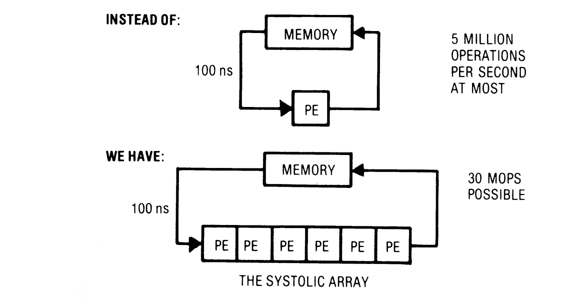
A systolic architecture is characterized by a network of processing elements (PE) that feed data to each other instead of going to the memory hierarchy for operands.
The core benefits are:
It alleviates memory bottlenecks by allowing multiple compute operations to occur without going to memory (as nicely depicted by the figure above). The design can allow computation time to be balanced with I/O if designed properly, avoiding one stalling due to the other.
It can create simple, regular designs → a modular setup that can be extended for different functions. It is relatively easy to write the RTL!
2D arrays can very easily be deeply pipelined (as we will see below), naturally taking advantage of algorithm concurrency.
The PE network can look like a 1D array (pictured above), 2D array (the most common today), or even other connections for specialized computations.
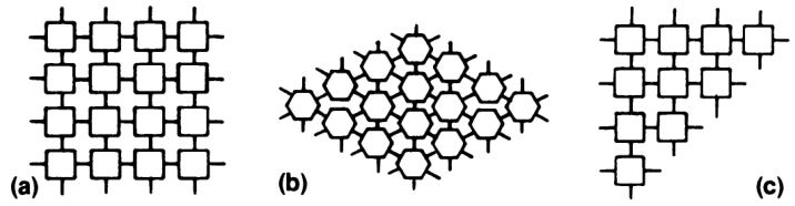
Data flows between cells in a pipelined fashion, and communication with the outside world is at boundary cells.
The foundation of TPU — a MAC systolic network
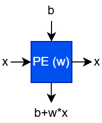
A multiply-accumulate (MAC) PE has two input edges and two output edges. In the form drawn below (“weight-stationary”), the weight w is a parameter loaded into the PE. The data x flows in and is passed unchanged left to right, and the current “accumulation” b flows in from the top (usually from a PE connected to the north). The PE does the multiply-accumulate (x * w + b) and passes the accumulated sum down. We assume that the calculation happens in a single “tick” or clock cycle.
A PE in a systolic network is typically a simple compute primitive. Its power comes from connections to other PEs to express complex calculations.
The easiest way to understand how a weight-stationary systolic array works is to understand how a dot product is computed. This is shown in the following image for 3 cycles, and we will walk through the computation.
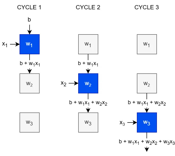
In each cycle, a new entry of x appears from the left, and one term is added to the dot product. The column of PEs contains a vector of weights. In each cycle, one term of the dot product is accumulated, and after 3 cycles, we have accumulated the full dot product b + w·x.
We now draw the exact same operation, but in an abridged form (not showing the intermediate calculations and instead just showing the inputs and outputs at the ticks they appear).
A column of the array is drawn as vector weight wi
The inputs are drawn as a diagonal (and enters the array skewed in time)
The output is shown at the bottom, appearing after R cycles from when the input hits row 1, where R is the number of PE’s in the column
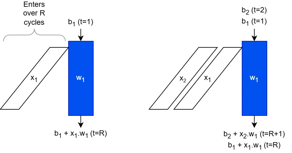
In this form it is easy to see that we are pipelining different xi by starting the second one the cycle after the first one. The initial accumulator value can be set to bi, an affine bias.
So, with a single column systolic array, holding a column vector w, we are computing y = b + X·w, where the rows of X are x1, x2, …
It is also noting the latency between when the xi starts getting input to when we receive the output: The first element of x1 enters the array at time t=1, and we get the result out at t=R, so the latency is R-1 cycles.
Making this a 2D array (recall that the input x’s are bypassed to the right from each PE), we see that xi will just arrive to interact with w2 one cycle later. We can appropriately skew the columns of the B matrix:
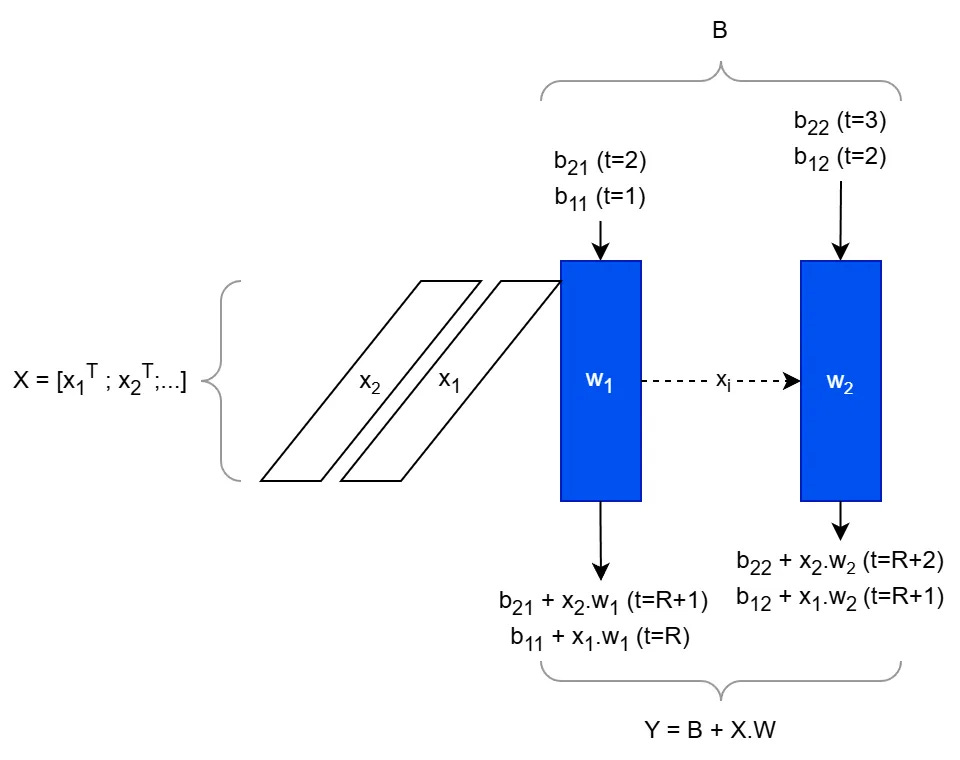
The operation that is executes is Y = B + X·W, where bij above is in row i and column j of B, W = [w1, w2] is the fixed weight matrix loaded in first. If W is n×n, and X is m×n, the matrix product is O(mn2) operations (as is standard), but due to the structurally-enforced pipelining, it was completed in O(m+n) cycles!
And just like that, with a very simple MAC-computing PE, we can build up the matrix multiplication hardware unit that is the core of most AI hardware accelerators.
There is much more to be said about how it is implemented in RTL, how it performs, how the matrix shapes affect utilization, the total latency, throughput and efficiency benefits. We will go over that and intuitive insights in an upcoming Chip Insights post. In the remainder of this article, we will turn our attention to other, more overlooked, uses of systolic networks in applications to broader AI, robotics, and numerical methods.
Moving beyond MAC
Keeping the exact same 2D array structure and the skewed input feeding, observe that we had two underlying binary operations: the PE (node) computed multiply (·) and the arrow (edge) computed sum (+). In general, the array will compute the result with those operators replaced by any counterparts: (x1⊙w1) ⊕ (x2⊙w2) ⊕ ⋯
I’ll be brief with these and list further reading below, and try to draw special attention to ones that are interesting for applications in robotics and AI.
1) Pattern matching (Kung group)
Using logical and (∧) and logical or (∨) as the operations: y = (x1∧w1) ∨ (x2∧w2) ∨ ⋯
This will return 1 if the vector x matches the vector w, and 0 otherwise.
2) Sorting (Kung group)
This one is fascinating and intuitive. Each PE performs a simple compare and swap operation, and passes the max downward and the min rightward. With n rows and n columns, it will execute the odd-even sort algorithm and produce the sorted array.
A glance at that wikipedia page reveals both a weakness and a strength of systolic arrays. They can only execute algorithms that can work based on local connections (the odd-even sort takes O(n2) operations, vs. more optimal algorithms), but as in matrix multiplication above, the latency is O(n). While the best sort algorithm takes O(n log n) steps sequentially in scalar hardware, the systolic network lets suboptimal algorithms complete with lower latency.
3) 2D motion planning
Deterministic motion planning (identifying environmental obstacles and planning a path through free areas respecting the system dynamics) is a fundamental problem in robotics. About 10 years ago there was even attempt to build chips to solve this problem.
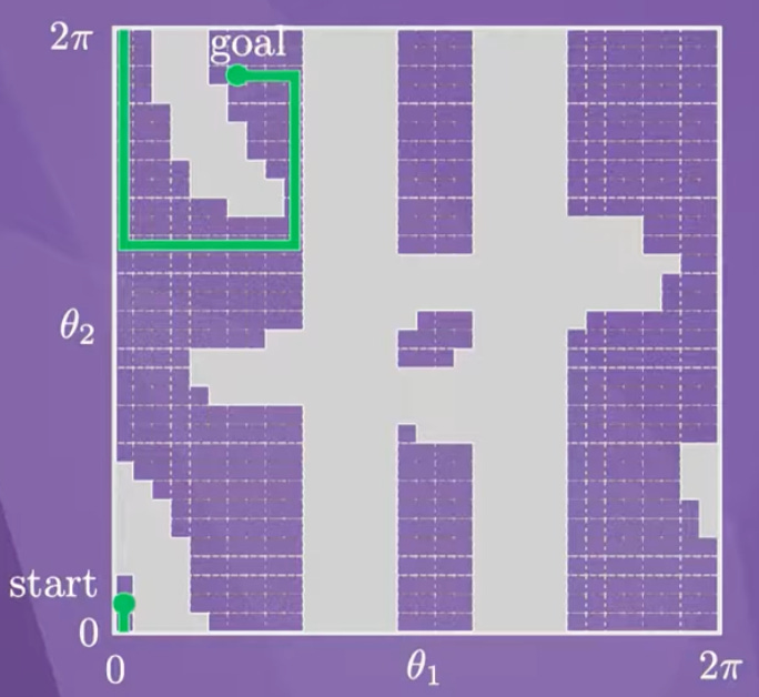
Dynamic programming solutions (including Dijkstra’s algorithm, A*) can be implemented by local and iterative propagation from the goal, and just as with odd-even sort, the nearest-neighbor connection pattern can be mapped well to a systolic array.
Unfortunately, the number of grid cells grows exponentially with the dimension of the ambient space, and this is problematic if we need to have one PE per cell. This makes systolic motion planning impractical unless we only have a 2D problem to solve, but I think it is an interesting application nonetheless.
4) Stereo vision semi-global matching
A PE that accumulates matching costs along a scanline can be used to form a systolic array that implements semi-global matching (SGM). This algorithm is used to calculate disparity in the very popular Intel RealSense camera ASICs.

SGM systolic arrays on FPGAs run this at pixel rate, processing one scanline per clock, and deterministic low-latency computation is obviously paramount here.
5) Matrix decompositions for numerical methods
To some extent, I’ve saved the most promising (at least in my view) for last. Matrix decompositions that aid in factorization are key to solving systems of equations, and this is ubiquitous in all sorts of robotics and general problems.
5.1) QR decomposition. This matrix factorization is the numerically stable way to solve least squares or pseudoinverses in overdetermined systems, and has applications to robot kinematics, SLAM, sensor fusion, online parameter estimation, etc. Additionally, it is a key component of quadratic program (QP) solvers: in active set solvers after the active set is identified, for Jacobian factorization in SQP, etc. These workloads are important in low-level control in robotics and typically need deterministic and low-latency solutions. The Givens rotations method (gentle explainer here) performs local operations on 2x2 submatrices, which lends itself very well to locally-connected CORDIC-implementing PEs in a systolic array.
5.2) Cholesky decomposition for symmetric positive-definite (SPD) matrices. This is a slightly easier factorization if the matrix is SPD, which comes up for example in state estimation, Kalman filtering, normal equations in interior point methods, etc. These workloads would come up in dedicated state estimation blocks in robotics pipelines. For decomposing A = LLT with lower-triangular L, each PE computes one entry of L using only its left and upper neighbors, making the data dependencies purely local. This is repeated on the smaller matrix till completion.
Both of the systolic implementations referred to above use non-MAC PEs, and a triangular (not rectangular) network — this is very uncommon in current hardware, but was represented in the Kung references above.
For this post, I wanted to stick to high-level intuitive descriptions, but in the open-source TinyXPU project, we will aim to implement and analyze some of these non-traditional systolic networks for robotics and AI pipelines. Stay tuned for the upcoming post introducing this project!
Conclusion
Systolic arrays were both invented before people think, and are more general than people think. They can have deterministic (no cache misses) high throughput and energy efficiency for algorithms which can work on local data. However, they are bad for working with sparse data (e.g. for sparse linear system solving), and bad for algorithms that need global data (e.g. Householder QR, which needs to operate on a full matrix column at a time).
In the deep neural network boom, the MAC array is so dominant in workload (>95% of operations in any DNN) that the non-MAC compute takes a tiny fraction of time. Dedicating a full systolic array with n2 PEs to non-MAC operations would be area-inefficient for neural net workloads. This is why commercial vendors have not explored the co-design of systolic networks with algorithms, including PEs that can do MAC but also other functions like Givens rotations on one chip. For robotics workloads and other general scientific methods, the mix of primitives is different and (in my opinion) worth revisiting.
Further reading
Kung 1982: Why Systolic Architectures - Great high-level overview of the motivation beyond systolic architectures
Kung 1982: VLSA Array Processors - Further detail on applications such as QR decomposition
Related posts:

