
Model-predictive control of RoboBee flapping flight
Hierarchical model-predictive and data-driven control method published in IJRR (2022)

In this post, we’ll go over a method to control the flight of a RoboBee in a way that should be approachable for a broad audience. In keeping with this publication’s focus on energy-efficient robotics, this method was designed to run on extremely low-power computational hardware, as we will see.
Just to provide brief context,
the RoboBee hardware was at this point fairly mature, and on the “Split Dual-Actuator Bee” generation;
the state-of-the-art flight controller was a capable, but task-specific hovering controller with limited generalizability.
The goal for this project was to develop a controller that could be easily generalized to more complex tasks using modern control methods. The resulting paper1 with Dr Rebecca McGill made some demonstrable advances in terms of better operation away from an upright configuration, the ability to stabilize tasks like following a desired path or executing more dynamic behaviors like perching and flipping, as well as robustness to suboptimal gain tuning and manufacturing variability.
Here are some hovering clips (short 32s video; no audio):
The remainder of this post explains how this result was achieved, and potential future extensions of the idea.
Background
RoboBee and flapping flight
The RoboBee is a 100mg flapping robot developed by Dr. Rob Wood, capable of hovering and controlled flight. To put it in perspective, a US nickel weights 5g or the equivalent of 50x RoboBees. Having spent a lot of time in the Harvard microrobotics lab fabricating them, it is no exaggeration to say that a sneeze can literally destroy weeks of work.
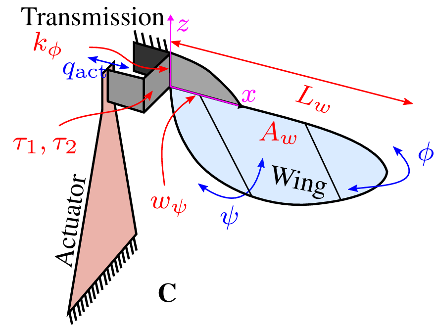
Along with a family of similarly-fabricated robotic systems developed at the Harvard microrobotics lab, they are actuated by piezoelectric bending actuators. The piezoelectric effect is commonly seen in the working of microphones, which convert vibrations created by acoustic pressure waves into electric signals. They also do that in reverse, converting electric pulses into vibratory motion. The RoboBee uses piezoelectric bending actuators, constructed similarly to a bimetallic strip, converting slight expansion and contraction of the piezoelectric material into a bending motion.
Generally, the piezoelectric actuators produce very small motions that need to be amplified to produce the requisite aerodynamic work. After the conversion to the bending motion, they also go through another transmission that converts the small bending translational motion into a rotational motion. In a previous post, I went into the details of how this transmission works, and a project I worked on to optimize it.

OK, now we are at the stage of converting electrical signals into rotational motion of the wing. The wing itself is attached to the end of the transmission via a passive hinge, so that when the base of the wing is flapped, it not only flaps, but also pivots about its hinge, thereby actively changing its pitch, or angle-of-attack. This motion is common among flapping animals:
RoboBee’s clever design allows the wing pitch to change passively as the wing flaps, i.e. only one actuator is needed per wing to obtain something resembling the complex wing motion of the hummingbird above:
Modeling RoboBee’s flight
A model of the motion produced is very important to understand how to use the available wing input signals to get to a desired goal. There is a large debate between model-based vs. model-free methods (which eschew models in gathering a lot of data with the black box system and approximating its behavior). Increasing computational power recently has resulted in increased temptation to abandon models, though in many sim2real reinforcement learning approaches, models are used in developing the simulation.
In the case of RoboBee, the difficulty with pursuing a fully model-based method is that aerodynamics is quite difficult to model. Nonetheless, some work in the early 2010’s on blade-element modeling has proved quite useful for understanding the relation of RoboBee wing motion to the produced lift and drag forces. Using that model, we developed a RoboBee simulator, which is open-sourced2. We will discuss the software supporting this work further below, but here is an animation of some fixed control inputs (similar to the 2013 flight control work) producing simulated flapping flight, complete with passive wing pitching (short 17s video; no audio):
The disadvantage of the model above that it is very complex and not possible to use to directly develop a controller. However, the other components of RoboBee dynamics (excluding how the wing produces lift and drag) are well-explained by Newtonian physics. In this latter area, there is a great degree of similarity to the control of legged robots.
Typically the world of flapping flight and legged control do not overlap, but there are a number of similarities that motivate the use of similar methods. They are both
cyclic (though in the RoboBee case, the wings are assumed massless and flap so fast that their dynamics are considered decoupled from the body);
mechanics-dominated (it is very important to consider the physics of ground interactions and aerodynamics); and
underactuated (we don’t have enough actuators to fully stabilize the motion, and typically in these scenarios some amount of “lookahead planning” is required).
In the legged robotics field, there is a long tradition of using simplified models to aid in control development (so-called “spring-mass” models), as I have discussed before. In this paper, we introduce for the first time an equivalent for RoboBee-like flapping flight.
Model-predictive control (MPC)
As discussed above, in underactuated scenarios, it is typically the case that some knowledge about the future behavior of the system can be predicted in order to decide which inputs to supply. As a simple example, how should the cart be moved in order to get the attached pole to swing up?
A global understanding of the future behavior of the system can be summarized in a so-called value function, and knowing this function can tell us exactly which way we should move to get to our goal from all states.
The problem is, the value function is not “known.” It can be estimated by exhaustively poking and prodding the system (which is an approach that resembles reinforcement learning). However, when we know of a dynamical model for the system, it is sensible to use it, because it greatly reduces the dimensionality of the control system to treat the dynamics as fixed.
Model-predictive control (MPC) tries to create a small local approximation of the value function online by using the future state of the system over a short prediction horizon (subject to a model) as a proxy for the value of the current state. MPC is now an old technique, but widely used in industrial process automation, aerospace, etc.
Approach: model-based MPC and model-free inverse dynamics
Here is the overall plan:
Develop a simplified model capturing the desired behavior: for this step, I noted that we do not care about the heading, but instead simply that the robot stays upright.
“Anchor” the behavior on to the RoboBee: convert to signals that get sent to the acuators.
The system architecture figure below makes this explicit. The purple “flying brick” is the model, whose future states we can predict for known inputs. The MPC can then effectively back out the best inputs for that model to get to a desired state.

However, as the blue and green arrows in the figure show, that only partially solves our problem because the RoboBee is not a flying brick. To address the gap, we need to define the operations undertaken by the arrows:
State projection (blue arrow): This process is relatively simple for this instance, because the state of the flying brick is effectively a subset of the state of the actual RoboBee. It has an elevation and body tilt angles just like the RoboBee, and we simply project the coordinates to those of the flying brick.
Inverse dynamics (green arrow): The other direction is more complex—in essence, we want to go from the abstracted thrust/roll/pitch torque inputs for the brick → RoboBee wing actuator signals. This process is complex because of a couple of reasons:
The mapping is much more complex than any kind of projection; for the various components:
Wing voltage → actuator motion (depends on piezoelectric actuator electrical and mechanical properties)
Actuator motion → wing base motion (depends on transmission and its stiffness)
Wing base motion → wing motion (depends on hinge and wing mechanical properties)
Wing motion → reaction forces and torques (depends on wing aerodynamic interactions, ground effect, etc.)
Manufacturing variability makes this mapping inexact (if you manufactured two RoboBees, they may require different wing signals to produce the same wing motion)
For these reasons, models have limited utility for the green arrows, and so, the paper proposed a model-free method for that part.
Model-based MPC
Template: upright rigid body
First, we need to pick the model. As the saying goes, all models are wrong, but the goal here is to capture the most important parts of the dynamics, and the objective.
The RoboBee’s wings are very light, and so most of its mass is truly contained in its body (more on this below). Dynamically, this is well-approximated by the flying brick, with no other moving parts.
To capture the objective, we note that we do not particularly care about the heading of the RoboBee when we just want it to hover, or fly controllably. This allows us to effectively remove one degree of freedom from our specification of the objective, and capture the state of the flying brick with:
To capture the position, we use the (x, y, z) Cartesian coordinates of the center of mass as expected.
To capture the orientation, we only look at the components of the “upright vector” (a vector pointing up in the body frame). Note that an objective of hovering can be simply stated as the desire to have the upright vector point vertically up.
Waypoint tracking MPC
We write the dynamical equations for the flying brick using the Newton-Euler equations for the motion of a rigid body. After a small approximation as described in the paper, we get
where p represents the Cartesian position, s represents the upright vector, T represents the (scalar) upward thrust, and τ represents the (2-dimensional) roll, pitch torque vector.
These equations are quite simple, owing mainly to the fact that the wings are quite light, and so their flapping does not significantly impact the motion of the much more massive body. This concept is also utilized in many legged running robots, referred to there as “massless legs.” It’s worth taking a minute to appreciate the significance of this: in practice, human limbs are not massless, which allows (for example) a gymnast to adjust their body orientation while flying through the air by controllably moving their limbs and landing a flip. However, mastering that kind of control is much more difficult than the massless legs (or wings) paradigm, where we can safely make the assumptions that the appendages simply produce a force or torque that acts on the body. A helpful picture to have in mind is that in the massless appendage paradigm, we can substitute the appendages for thrusters attached at appendage base, and pretend we are controlling the thrust vector instead.
Upon further inspection, the equations are second-order (as expected for any mechanical system). The orientation equation is also unfortunately nonlinear, as can be seen from the product of s, T, and τ appearing on the right side. This is also normal for such systems, but adds a challenge to our MPC transcription.
To resolve this difficulty, we linearize these dynamics at the current orientation and thrust (s0, T0) before incorporating them into the model-predictive controller. The controller will reason about the best inputs based on how they act on the current state, which intuitively is fine for a short enough planning horizon.
As an analogy, a car driver on the highway will turn their steering wheel slightly to change lanes (an action that is appropriate for a planning horizon for a few seconds), even though that action would not be appropriate on a long enough horizon that they drive off the highway. Similar to the car driver, the RoboBee in this scenario will re-evaluate its inputs with a new state soon enough. MPC always works this way, with a finite planning horizon a short duration from the current time.
The objective for the MPC is to track a trajectory of future states, including a position and velocity. For example, to hover, the desired position is the hovering goal position, and the desired velocity is zero. To follow a particular path in space, that path can be discretized and substituted into the desired positions.
Simulation evaluation
To evaluate if the MPC with the linearized dynamics above works appropriately, we can compare the performance of the controller in a number of simple tasks in an apples-to-apples comparison with the prior state-of-the-art reactive controller.
Hovering, trajectory following

The tasks, as shown above, were:
Hover task starting off withan initial orientation with roll and pitch angles set to 0.5 rad, -0.5 rad, and initial velocity 0.1 m/s in the x-direction
Waypoint tracking on an “S”-shaped trajectory in the xz-plane.
Tracking a commanded velocity of 2m/s for 0.5 seconds before stopping.
In each of these scenarios, the MPC performs better than the reactive controller (notes on tuning below), which is promising.
Perching, flipping
Specifying a task in terms of a reference trajectory can be onerous, for example, if we want the bee to do a backflip, it isn’t clear what sequences of positions and velocities are appropriate for the horizon.3 To test the robustness of the MPC, here we feed it “made up” infeasible trajectories and see how well it can track them.
The tasks we choose to test include the aforementioned flip, and a wall-perching behavior inspired by this past research:
The reference trajectories are selected intentionally naively:
For the perch task, the desired position translates smoothly to the right, and the desired orientation steadily rotates to 90 degrees at the end of the motion
For the flip task, the desired position is fixed, and the desired orientation smoothly rotates 360 degrees.

The results show that the MPC is able to compensate for the naiveté of the reference trajectories to accomplish the task to satisfaction. The reactive hover controller cannot solve these tasks.
A note on tuning the controllers
Something that most research papers will sweep under the rug is the process of how the controllers were tuned. The previous state-of-the-art reactive controller has hand-tuned PD gains, and the MPC has weights on the objective. To make a fair comparison, we have to tune both as best as possible.
In general, there is a tradeoff between tracking error and tracking effort. As an analogy, cruise control in cars often have an eco mode, where they may deviate from the speed setpoint a bit more, but waste less fuel. Similarly, you can spend less actuator effort in exchange for tracking the goal a little less precisely. This is usually one of the ways in which controllers are tuned in practive.

The plot on the right shows the MPC and the reactive controllers fairly compared with a variety of tuning gains, showing that the MPC is significantly easier to tune, and can track better with lower actuator effort than is possible with the reactive controller.
Data-driven inverse dynamics
As we discussed above, the mapping from actuator signal → produced force/torque is unknown/uncertain due to the system complexity and manufacturing variability.
An example of a common type of manufacturing variability is that some RoboBee transmissions just exhibit higher stiffness than others. If the left wing has a stiffer transmission than the right wing, the left wing may flap with a smaller wing amplitude than the right one when driven equivalently, and produce much less lift force.
In this project we took the approach of breaking down the components of this mapping, and just using data to characterize the variable parts. This meant collecting data of wing kinematics as a function of actuator signals and then fitting a function to approximate some “kinematics features” that could be expected for each actuator signal:

We then used the blade-element model to predict the reaction force/torque from the wing kinematics.
To show the effect of this kind of mapping, we performed the same operation in the RoboBee simulator, and simulated the effect of adding a force bias of 3 mN to one of the actuators. With no force bias, the data-driven mapping and the manually-tuned mapping both work, but with the force bias, the data-driven mapping can still work while the manually-tuned mapping fails.

Hardware integration
Setup
Encouraged by the simulation results, we pushed ahead to integrate the MPC into the physical RoboBee control system, which looks as follows:

The actuators were connected to a Simulink real-time control PC, which was new to me. The setup encourages code to mostly be compiled from graphical blocks such as filters, delays, etc., but does allow for custom blocks written as MATLAB functions. While the state estimator and some other components were in fact MATLAB functions, we implemented the MPC in C using OSQP, as part of a more forward-looking architecture that could also run onboard the RoboBee on a microcontroller.
When run from the Simulink target PC, the iteration frequency was 5KHz for everything, locked together due to the Simulink architecture. The MPC itself also ran at 100-200Hz on small STM32G4 MCU that fell within the 25mg payload constraints of the RoboBee. We tested that the controller could successfully stabilize the simulator when run at rates of 100Hz.
Experimental results for hovering
A video clip of some of the hovering results were linked to in the introduction of this post. Some overlaid trajectories from those trials are shown in the figure below.
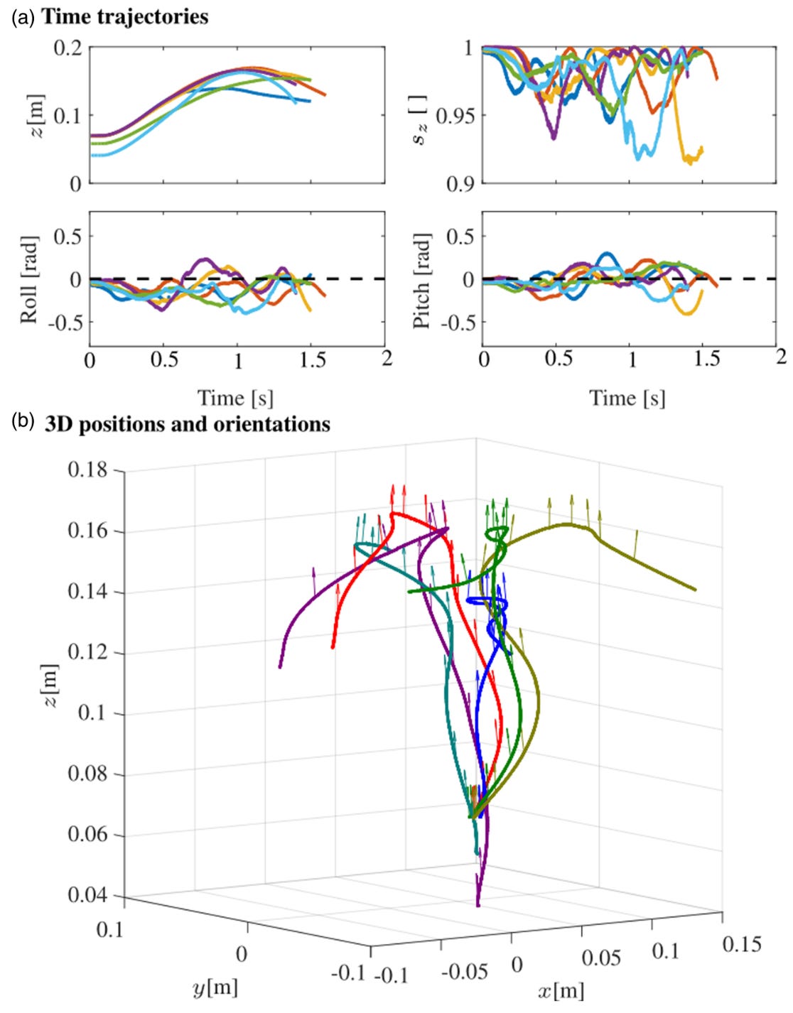
Each trial ended due to the motion capture system losing track of the RoboBee, or by a command we sent. We were able to keep the orientation stabilized in each trial, though the horizontal position drifted more than desired.
The hovering task was overall a good demonstration of the feasibility of integrating this much more advanced controller paradigm into the RoboBee.
In the future, it would be very exciting to see either or both:
some of the tasks we tested (and compared to the reactive controller) in the simulation section running on the RoboBee
the controller running on a microcontroller, along with onboard sensing and power, for fully untethered complex flight
Implementation details and replicating results
In the interests of open science, the code for various parts of this project are all online. While I don’t have continued access to the Simulink software and experimental setup, if you need support, please comment below—continued progress and replicability are well worth the support and debugging.
MPC
This is implemented as a quadratic program with OSQP.
The quadratic program is defined in genqp.py. When that file is run as a script, it instantiates the controller and runs a test, or in the commented-out section at the bottom, run’s OSQP’s codegen feature to generate a standalone set of C files that can solve the QP. The codegen output is stored in the uprightmpc2 directory (though it can be regenerated as well).
The codegen outputs define the structure of the problem, but the variables need to be updated as the current state of the RoboBee or the reference trajectory changes. To do this, the uprightmpc2.h file provides some simple interfaces with named parameters that can be called. The C file of the same name contains its implementation.
The C code in the uprightmpc2 file can be built using CMake; something like
cd uprightmpc2
mkdir -p build && cd build
cmake ..
Simulations
The simulations testing the MPC with the upright template model can be run from the template directory.
The uprightmpc2.py file should recreate the test scenarios covered in plots above and in the paper when run as a script. The bottom of the file contains code describing the test scenarios that can be uncommented.
The 3D pybullet simulation can be run by executing the robobee.py script.
Simulink setup
The C code is integrated into the Simulink real-time setup as an S-function; the legacy_code_gen.m file configures the inputs and outputs of the block that will appear in Simulink. See this page for more guidance on this process, which was quite tricky.
The simulink model files are slx files, and can be found here.
In practice, for these kind of tasks, it is common in the state-of-the-art to use offline optimization or learning (which takes much more computation to run) to figure out the best trajectory, and then use that reference for the MPC.